Reason 2 It’s easy to get started
- Installing R and RStudio
- Creating a new project in RStudio
- Running commands in the R console and from a script file
- R’s basic operators
- Using functions
Getting R to run on your computer is usually a relatively smooth experience9: Download and install the latest version of R (https://r-project.org/) and RStudio (https://rstudio.com/products/rstudio) for your operating system. If you already have either program installed on your computer, there is no need to uninstall the old versions beforehand.
If you cannot or do not want to install anything on your machine, you can instead make an account at RStudio Cloud (https://rstudio.cloud/). This lets you to use R and RStudio in the browser. You can use RStudio Cloud for free for a few hours each month. For the purpose of working through this book that should be enough.
That’s it! Everything else you need can be set up from within RStudio.
Additional Software
If you are using Windows, you might eventually also have to install RTools (https://cran.r-project.org/bin/windows/Rtools/). This includes additional tools, such as a C/C++ compiler, that you will need for things like Bayesian statistics.
For reproducible research, you should also install Git (https://git-scm.com/), a version control system which we will briefly talk about later. For now, you do not have to worry about these things, because you can always do them later.
Exercise 2.1 Use one of the methods suggested above to get access to R and RStudio so you are ready to follow along for the rest of the book.
2.1 Why RStudio?
You might be wondering what RStudio is and why we need it. RStudio is a popular Integrated Development Environment (IDE) for R. It is an all-in-one user interface that provides many conveniences that make working with R a lot easier. To use an analogy: If R were a horse, RStudio would be a saddle to sit in. You don’t need it, but it makes things more comfortable. There are good alternatives to RStudio, but R’s own GUI is not really one of them:
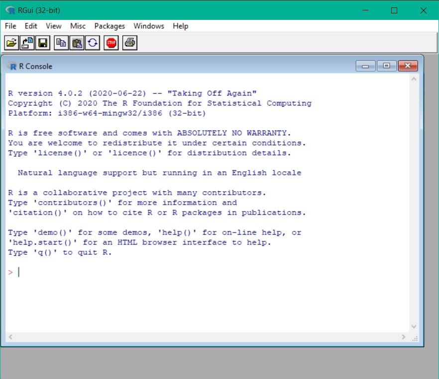
Figure 2.1: R’s own GUI — The 90s called, they want their user interface back.
2.2 Create a new RStudio project
Alright cowboy, let’s saddle that horse! 🤠
The first step you should do whenever you start a new data analysis project with RStudio is to create an RStudio project in a new folder. This is the first step towards reproducibility: All of your project’s data and files will be stored in this folder. If you ever move the project folder to a new location or share it with someone else, all of the files will move along with it, reducing the chance that things will break. Another benefit of using projects is that it helps you to keep your work organized. It will be much easier for you to switch between projects or get back to a project you haven’t touched in a while.
Exercise 2.2 Open RStudio, go to File ▸ New Project... and create a new RStudio project in an empty
folder. Leave Use version control and Use renv unchecked for now — we will get back
to those later.
Now that we have our project set up, let’s have a look around RStudio. The many panels and tabs in RStudio may be overwhelming at first, but I promise this gets better over time, and most of them are actually quite helpful. The console, for example, allows you to interact with R directly.
Figure 2.2: RStudio’s user interface with the four panels
2.3 Using R as a calculator
The console is the panel on the bottom left, the one with the expectantly blinking cursor. In the console you can type commands and when you press Enter, R will try to interpret them. You can also use ↑ and ↓ to cycle through previous commands and Ctrl/Cmd + ↑ to search through previous commands.
Using operators
Let’s get familiar with the console by trying some of R’s mathematical operators. R has all the operators that you would expect to find in a pocket calculator:
| Arithmetic | + - * / ^ |
| Modular arithmetic | %% %/% |
| Relational | < > <= >= == != |
| Logical | && || ! | & |
| Parentheses for modifying precedence | (1 + 2) * 10 |
Using functions
It also has all the functions you would expect to find in a calculator. Functions are
written as the function name followed by the function’s argument in parentheses. For
example, for calculating the square root of 2, use sqrt(2).
If a function has multiple arguments they will be divided by commas, as in
log(2, base = 10), which will give you the logarithm of 2 to the base of 10. Note, that
we supply the base as a named argument. Functions expect arguments in a certain order.
By using named arguments you can override this order, and you can supply individual
arguments while using the default value for other arguments (e.g., the default for
base in the log() function is Euler’s number \(e\)). This is common for functions with
multiple arguments. In our example, using the named argument isn’t really necessary,
because we are providing the arguments in the expected order, but it may still help to
make your code more readable.
Exercise 2.3 In the console, try out some of R’s operators and see what happens. For example,
What does
1 != 1.0do?What happens if you run an incomplete command like
1 *What happens if you run a command that does not make sense, like
1*/ 3
R checks whether the argument on the left side (
1) is not equal to the argument on the right (1.0). It returnsFALSEbecause to R these two numbers are identical.R waits for you to finish the command. Press Esc to terminate the incomplete command.
R throws an error message and tries to tell you what went wrong. If you are working with R, you will have to get used to getting lots of error messages.

Figure 2.3: Don’t worry – you can’t hurt R, it has been through this before…
2.4 Create a script
The console is useful for running quick throw-away commands, and sometimes that’s all you need. However, code that you want to keep should be stored in a script. We will use a special type of script, called an RMarkdown Notebook.
RMarkdown allows you to do literate programming. That is, it lets you mix code and the output the code generates with text. The text can be formatted with a special syntax to create headings, footnotes, links, and more. This allows you to keep your notes and your code together and is great for writing reproducible documents. In fact, this entire book was written with RMarkdown.
Exercise 2.4 Go to File ▸ New File ▸ R Notebook to create a new RMarkdown Notebook and save it in
your project’s working directory as analysis.Rmd. Note that the file has appeared in
RStudio’s Files tab, which shows you the content of your project folder.
The new notebook already contains some example content. You can see that there is R code that is written inside special blocks, called code chunks. You can create new code chunks with the green button on the top right of the script panel or with the keyboard shortcut Ctrl/Cmd + Option/Alt + I
R scripts still allow a flexible console-like workflow because you can run individual sections or lines of code in any order. You can…
- run an entire code chunk by clicking the green arrow on the right of the chunk.
- run individual lines or sections of code by using Ctrl/Cmd + Enter or the buttons on the top right of the script panel.
Exercise 2.5 Add a new code chunk to your R Markdown Notebook in which you calculate the square of
2021 as well as the square root of 1764. Then run the chunk.
The code chunk in analysis.Rmd should look like this.
```{r}
2021^2
sqrt(1764)
```
When you run the chunk, the output should be
[1] 4084441
[1] 42
It can be more complicated if you are working on a machine with restricted permissions, for example a computer issued to you by your employer. If you are in a situation like this, and you are experiencing problems with the installation, please contact your IT department to sort it out.↩︎